Find Non-trivial Solution to Linear Equations in Sympy
How do you use NumPy, SciPy and SymPy to solve Systems of Linear Equations?
Let's solve linear systems with a Unique solution, No solution or Infinitely many solutions
![]()
In linear algebra, a system of linear equations is defined as a collection of two or more linear equations having the same set of variables. All equations in the system are considered simultaneously. Systems of linear equations are used in different sectors such as Manufacturing, Marketing, Business, Transportation, etc.
The solving process of a system of linear equations will become more complicated when the number of equations and variables are increased. The solution must satisfy every equation in the system. In Python, NumPy (Numerical Python), SciPy (Scientific Python) and SymPy (Symbolic Python) libraries can be used to solve systems of linear equations. These libraries use the concept of vectorization which allow them to do matrix computations efficiently by avoiding many for loops.
Not all linear systems have a unique solution. Some of them have no solution or infinitely many solutions.
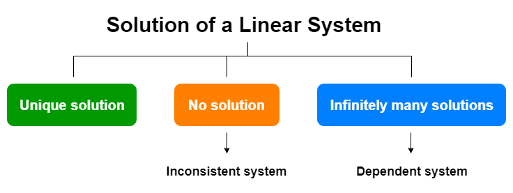
We will cover these 3 types of linear systems with NumPy, SciPy and SymPy implementation. The implementation can be done in a few different ways. We'll also discuss these different ways where necessary. At the end of this article, you'll be able to solve a linear system (if a unique solution exists) and identify linear systems with no solution or infinitely many solutions with powerful NumPy, SciPy and SymPy libraries.
Prerequisites
Basic knowledge of NumPy (array creation, identification of one-dimensional and 2-dimensional arrays, etc) is highly recommended. If you're not familiar with them, don't worry. To get the basic knowledge, you can read the following article written by me.
Let's get started!
An example of a linear system
Have look at the following image which contains a linear system of equations.
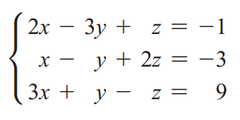
There are 3 linear equations in this system. Each equation has the same set of variables called x, y and z. Solving this linear system means that finding values (if exists) for x, y and z that satisfy all the equations.
Matrix representation of a linear system
The above system of linear equations can be represented as a special matrix called the augmented matrix which opens the path to solve linear systems by doing matrix calculations.
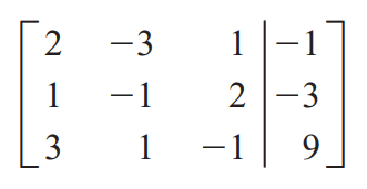
There are two parts of this augmented matrix:
- Coefficient matrix — This is a rectangular array which contains only the coefficients of the variables. In our example, this is a 3 x 3 square matrix left of the vertical line in the above picture. The first column contains the coefficients of x for each of the equations, the second column contains the coefficients of y and so on. The number of rows equals the number of equations in the linear system. The number of columns equals the number of different variables in the linear system. In NumPy, this can be represented as a 2-dimensional array. This is often assigned to a variable named with an uppercase letter (such as A or B).
          import numpy as np          A = np.array([[2, -3, 1],
            [1, -1, 2],
            [3, 1, -1]])
- Augment — This is a column vector right to the vertical line in the above picture. It contains constants of the linear equations. In our example, this is a 3 x 1 column vector. In NumPy, this can be represented as a 1-dimensional array. This is often assigned to a variable named with a lowercase letter (such as b).
import numpy as np b = np.array([-1, -3, 9])
Solving linear systems with a unique solution
Let's solve the following linear system with NumPy.
To solve this right away, we use the solve() function in the NumPy linalg subpackage.
          import numpy as np          A = np.array([[2, -3, 1],
            [1, -1, 2],
            [3, 1, -1]])          b = np.array([-1, -3, 9])          np.linalg.solve(A, b)
The output is:
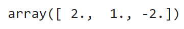
Wow! The above linear system has a unique solution:
- x = 2
- y = 1
- z = -2
Note: A similar type of implementation can be done with SciPy:
from scipy import linalg linalg.solve(A, b)
How does this work internally?
The direct implementation does not give a clear idea of how this works internally. Let's derive the matrix equation.
Matrix Equation

Let's get the same solution using the matrix equation:
np.dot(np.linalg.inv(A), b)
To have a solution, the inverse of A should exist and the determinant of A should be non-zero:
np.linalg.det(A) 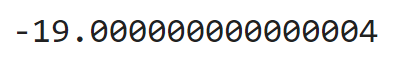
Solving linear systems with no solution
When a system of linear equations has no solution, such a system is called an inconsistent system. Let's see what will happen when we try to solve the following linear system with NumPy:
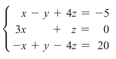
          import numpy as np          A = np.array([[1, -1, 4],
            [3, 0, 1],
            [-1, 1, -4]])          b = np.array([-5, 0, 20])          np.linalg.solve(A, b)
The output is:
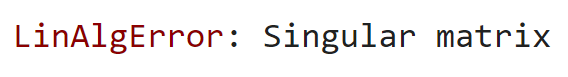
The error message says that our coefficient matrix (A) is singular. In algebra terms, it is a non-invertible matrix whose determinant is zero. Let's check it:
np.linalg.det(A) The output is:
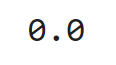
The determinant is zero. Therefore, our coefficient matrix (A) is singular. Because of that, the above system of linear equations has no solution!
Note: If you implement this with SciPy, a similar type of error message will be returned.
Solving linear systems with infinitely many solutions
When a system of linear equations has infinitely many solutions, such a system is called a dependent system. Let's see what will happen when we try to solve the following linear system with NumPy:
          import numpy as np          A = np.array([[-1, 1, 2],
            [1, 2, 1],
            [-2, -1, 1]])          b = np.array([0, 6, -6])          np.linalg.solve(A, b)
The output is:
This is the same as the previous case.
Note: If you implement this with SciPy, a similar type of error message will be returned.
Now, there is a question. How can we distinguish between linear systems with no solution and linear systems with infinitely many solutions? There is a method.
We attempt to put the coefficient matrix into the reduced row-echelon form which has 1's on its diagonal and 0's everywhere else (identity matrix). If we succeed, the system has a unique solution. If we are unable to put the coefficient matrix into the identity matrix, either there is no solution or infinitely many solutions. In that case, we can distingush between linear systems with no solution and linear systems with infinitely many solutions by looking at the last row of the reduced matrix.
Getting the reduced row-echelon form
We can use the SymPy Python package to get the reduced row-echelon form. First, we create the augmented matrix and then use the rref() method. Let's try it out with a linear system with a unique solution:
          from sympy import *          augmented_A = Matrix([[2, -3, 1, -1],
            [1, -1, 2, -3],
            [3, 1, -1, 9]])          augmented_A.rref()[0]
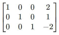
We succeeded! We got the reduced row-echelon form. The 4th column is the solution column. The solution is x=2, y=1 and z=-2 which agrees with the previous solution obtained using np.linalg.solve().
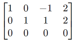
Let's try it with a linear system with no solution:
          from sympy import *          augmented_A = Matrix([[1, -1, 4, -5],
            [3, 0, 1, 0],
            [-1, 1, -4, 20]])          augmented_A.rref()[0]
In this time, we did not succeed. We didn't gt the reduced row-echelon form. The 3rd row (equation) of this form is 0=1 which is impossible! Therefore, the linear system has no solution. The linear system is inconsistent.
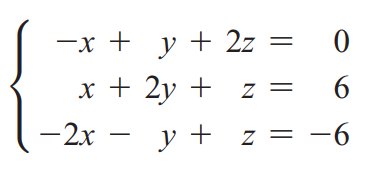
Finally, we try it with a linear system with infinitely many solutions:
          from sympy import *          augmented_A = Matrix([[-1, 1, 2, 0],
            [1, 2, 1, 6],
            [-2, -1, 1, -6]])          augmented_A.rref()[0]
In this time also, we did not succeed. We didn't gt the reduced row-echelon form. The 3rd row (equation) of this form is 0=0 which is always true! This implies the variable z can take any real number and x and y can be:
- z = any number
- x-z = 2 (x = 2+z)
- y+z = 2 (y = 2-z)
By substituting any real number to z, we can get infinitely many solutions! The linear system is dependent.
We've done the job. Now, you're able to solve a linear system (if a unique solution exists) and distinguish between linear systems with no solution and linear systems with infinitely many solutions with powerful NumPy, SciPy and SymPy libraries.
The general implementation is:
First, try np.linalg.solve(). If you get a unique solution, you've done the job. If you get an error message ("Singular matrix"), the linear system either have no solution or infintily many solutions. Then, try to get the reduced row-echelon form using SymPy Python package as discussed above. By looking at the last row of he reduced form, you can decide the things!
Also, note the following points too.
- The above-discussed methods can only be applied to linear systems. In other words, all the equations in the system should be linear.
- If a linear system has fewer equations than variables, the system must be dependent or inconsistent. It will never have a unique solution.
- Linear systems with more equations than variables may have no solution, unique solution or infinitely many solutions.
Find Non-trivial Solution to Linear Equations in Sympy
Source: https://towardsdatascience.com/how-do-you-use-numpy-scipy-and-sympy-to-solve-systems-of-linear-equations-9afed2c388af